Want code? Click here.
Attempting to Train Stable Diffusion From Scratch For Free
A comprehensive description of my thoughts when trying to make a latent diffusion model (LDM) train as fast as it can while only free compute sources
Written by latentCall145 on August 17, 2023 and published to this site on September 2, 2024 (changelog)
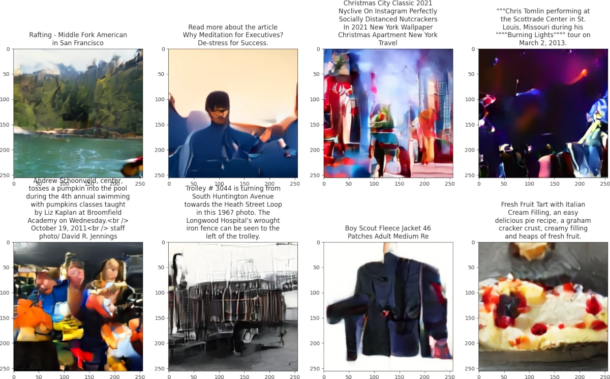
Non-cherry-picked generated outputs after 90k steps at batch size 1024, lr=1e-4, ~25 million img subset of laion2B-en.
Introduction
I always wanted to know how Stable Diffusion worked. So, I've been working on this project since last year but I had to put a hold on it because of school, but I resumed it this summer. I implemented the VAE and DM training and got some results before I held the project, so this summer I wanted to make a version which:
- Is free of cost
- Gives reasonable image outputs for a text input
- Trains fast
| Compute Provider | GPU Compute | TPU Compute | Time per interactive session (hours) | Quota per week (hours) |
|---|---|---|---|---|
| Colab | T4 (V100 on rare occasions) (16 GiB) | TPU-v2-8 (8 GiB / device) | < 4 | like 10-20? |
| Kaggle | P100 (16 GiB, no mixed precision) OR 2 x T4 (16 GiB / device) |
TPU-v3-8 (16 GiB / device) | 9 | 30-40 (GPU) 20 (TPU) |
| Paperspace | M4000 (8 GiB, no mixed precision) | N/A | 8 | varies on GPU availability |
Of these three, Kaggle provides both the fastest hardware for GPU and TPU, the longest interactive session time, and the longest quota out of all the options. In general, when training large models, Kaggle is the only good compute option. Kaggle also provides users to create unlimited datasets.
Goal 2 was also relatively easy. Since I had a training script which could train an LDM (latent diffusion model, this is Stable Diffusion's architecture), I just had to train longer on more data. So I 10x-ed my dataset, from 80 GB (~2.56 million images) of images resized to 256x256 to 800 GB worth of images from the LAION-2.6B-en dataset (collected with img2dataset). Even with 10x the data, 25.6 million images is still tiny compared to the full LAION-5B or even the LAION-400M dataset, so I wouldn't know if I had enough images until I trained the DM for a while.
Goal 3 is the interesting one. To train a big model fast, the best free option that I have is Kaggle's TPU-v3-8 because it contains 4 chips (each with two cores, 4 chips * 2 cores/chip = 8 cores so TPU-v3-8), each chip having 123 TFLOPs of bfloat16 compute (so 4 chips * 123 TFLOPs/chip = 492 TFLOPs) [1] as compared to the P100's 10.6 TFLOPs [2] and the T4's "65 TFLOPs in mixed precision" [3] even though from my experience, a T4 using mixed precision is only slightly faster than a P100 in real-world training. Let's just assume that a T4 has 11 TFLOPs of mixed precision compute so two T4s has 22 TFLOPs, meaning that a TPU-v3-8 can be up to 22.4x faster than the fastest GPU combination freely available! TPUs it is.
But TPUs come with some of their own problems.
- TPUs have been very difficult for me to utilize effectively. While a TPU at 10% FLOPs utilization is still 2.24x as fast as two T4s, I literally have never seen TPU utilization go above 40% in any of my previous projects. However, part of this project was to understand how to get the monster FLOPs utilization seen in other large models (e.g. 54.9% model FLOPs utilization over 1024 TPU-v4s in ViT-22B [4, 5]), so I welcomed this challenge.
- Kaggle TPU availability varies on the time of day and during peak usage hours (generally 2-8 PM UTC), you may have to wait up to two hours to get a hold of one.
- TPUs require models to be compiled via XLA to be run. For the LDM that I trained (508 million parameter UNet), it takes around 30 minutes before the model actually trains on the TPU which makes profiling the model slow and painful.
- Although I'm using torch_xla, XLA runs via TensorFlow which is notorious for having errors that make zero sense and generally being hard to debug.
- Kaggle can't seem to control TPU sessions very well. Sometimes I run all notebook cells but some cells choose not to run so I have to rerun all notebook cells. Often I cancel a cell's execution and it doesn't stop unless I cancel it twice. Nearly every time I restart a session, Kaggle doesn't let me run any cells unless I restart it again. Most infuriating of them all, sometimes XLA runs into an error (usually an OOM) and the notebook just hangs. I cancel the cell execution, and nothing happens. I restart the session, and nothing happens. I restart it again, and nothing happens. The ONLY way I found to get around this situation is to factory reset the notebook, which sucks when you waited an hour to get a TPU session, wait 30 minutes for the model to compile, run into an error which hangs the notebook, and then now you have to wait another hour to have the factory reset-ted session to start running because you're working during TPU peak hours so you're #27 in the TPU queue. All of this happens exclusively on Kaggle TPU sessions.
But TPUs are fast, so I'll work with it.
Optimization Tricks
Note: These are ordered from when I found them.
Logging loss every 32 steps (instead of every step)
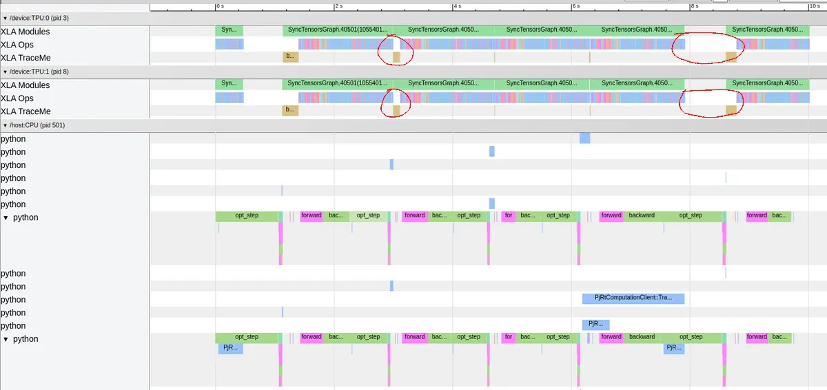
The PyTorch XLA guide states to log every N steps [10] and in general, when accessing the loss' values for logging, there is a TransferFromServer (TPU → CPU) event which adds some idle time. I chose 32 steps since that means that losses would be logged every one or two minutes, which is as often as I'd like without adding too much idle time.
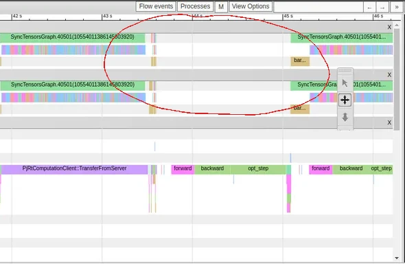
The trace viewer showing idle time (circled in red) caused by logging loss. Notice the purple TransferFromServer call before the idle time which gets called every time the loss is logged.
Writing my own multi-head attention PyTorch module
I initially made my own module over using PyTorch's MultiheadAttention layer because I wanted to be able to swap the scaled dot product attention portion with FlashAttention2 [6], which is both faster and uses less memory than PyTorch's attention function, which uses either xFormers or the 1st-gen FlashAttention. Also, PyTorch's MultiheadAttention takes in three inputs (query, key, value) when most of the time I'm running self-attention so I wanted an attention module which takes either one (self attention) or two inputs (cross attention). This allows for a simpler implementation for the model's forward passes. But it turns out that my custom module actually runs slightly faster on GPU and TPU and with slightly less memory usage! I'm not entirely sure why, but I'll take it.
Using SiLU instead of GELU
Stable Diffusion uses the GELU activation function so I copied it in my models. But when profiling and viewing the graphs of some test models which used GELU (e.g. a single transformer block), I noticed that there was a complicated operation which I realized came from GELU. This is because GELU is a pretty weird function [7] which doesn't seem to have primitive ops on a TPU (although it is optimized on GPU). While using the tanh approximation of GELU did increase my FLOPs utilization, I got even more from just using the SiLU activation function, which is just x * sigmoid(x), which is optimized on TPU since sigmoid is an XLA primitive op. This probably also explains why ViT-22B and PaLM use SwiGLU instead of GEGLU [4, 5] even though GEGLU allows for a slightly lower loss when training [8].
Splitting heads smarter
PyTorch's scaled dot product attention function takes inputs of shape (B, H, L, D) where B = batch size, H = number of heads, L = number of tokens, D = dimension per head. Let's call these dimensions after their size, so the attention input has the dimensions B, H, L, and D. Multi-head attention inputs are generally shaped (B, L, H*D) so I needed to rearrange these tensors before feeding them into the scaled dot product function. At first, I did:
def slower_split_heads(x):
    splitted = x.reshape(B, L, D, H) # B L (D*H) → B L D H
    return splitted.permute(0, 3, 1, 2) # B L D H → B H L D; this can be fed into torch.nn.functional.scaled_dot_product_attention
However, a slightly better way to do this is:
def faster_split_heads(x):
    splitted = x.reshape(B, L, H, D) # B L (H*D) → B L H D
    return splitted.permute(0, 2, 1, 3) # B L H D → B H L D; this can be fed into torch.nn.functional.scaled_dot_product_attention
The difference lies in the permute arguments, as the faster function preserves the relative ordering of the input's dimensions (i.e. which dimensions come before others) as best as possible. To clarify, in the faster function, notice how H comes before D in the tensor named "splitted" and in the returned tensor (ignoring any dimensions between H and D). This is not the case in the slower function, as D comes before H in "splitted" but H comes before in the returned tensor. In general, the fastest permutations are the ones where the relative ordering of the input's dimensions is similar to the relative ordering of the output's dimensions. I'm pretty sure this is because of cache locality; it's out of the scope for this project but here are some references if you're not aware of it and are curious: [12, 13, 14]
Avoiding torch.split like the plague
The TensorFlow TPU performance guide states to avoid unnecessary slices (and concatenations) [11], and since torch.split is a function that slices a tensor, it's not that fast on TPUs. I didn't learn to avoid torch.split from the TensorFlow TPU guide since I was on PyTorch, but while profiling my multi-head attention module, I was surprised to see a performance increase when I essentially changed:
def slower_self_attention(x): # BEFORE
    qkv_proj = nn.Linear(embed_dim, 3*embed_dim)(x)
    q, k, v = torch.split(qkv_proj, embed_dim, dim=1)
    # scaled dot product attention and linear projection

def faster_self_attention(x): # AFTER
    q = nn.Linear(embed_dim, embed_dim)(x)
    k = nn.Linear(embed_dim, embed_dim)(x)
    v = nn.Linear(embed_dim, embed_dim)(x)
    # scaled dot product attention and linear projection
Apparently, having three Linear layers is faster than using torch.split, so I removed nearly all instances of torch.split. This includes the QKV projections as shown above but also the gating mechanism in the SwiGLU layer:
def slower_swiglu(x): # BEFORE
    lin_gate = nn.Linear(channels, 2*channels)(x)
    lin, gate = torch.split(lin_gate, channels)
    return lin * torch.nn.functional.silu(gate)

def faster_swiglu(x): # AFTER
    lin = nn.Linear(channels, channels)(x)
    gate = nn.Linear(channels, channels)(x)
    return lin * torch.nn.functional.silu(gate)
I still use torch.split when splitting the VAE output into mean and log-variance tensors since I realized I used it after I trained the VAE, but I doubt causes much slowdown since this shouldn't take much time to execute and is only called once per training step).
Removing biases in transformer blocks
I heard that people started removing biases in transformers [17] and it gave me about 3% more FLOPs utilization when profiling transformer layers so I did it... not much else to it.
Modifying VAE and DM architecture to be TPU-friendly
When checking Tensorboard traces while training these unmodified networks, I saw that VAE inference took the vast majority of the computation. This is because I had my VAE and DM perform 16x and 8x downsampling respectively, which means that a 256x256 image would eventually be downsampled into a 2x2 tensor. This is ... really small. The less computation there is to do, the worse that GPUs/TPUs can be utilized, so downsampling images to 2x2 is not a good idea.
Small model = bad FLOPs utilization
Instead, the modified VAE had 8x downsampling with 4x less latent channels (16x16x16 → 32x32x4 latent, by the way this is the latent size described in the LDM paper), and the modified DM had 4x downsampling. Now, the smallest tensors in modified DM will still have an 8x8 spatial dimension, meaning that TPUs can run convolutions more efficiently on them. Also, the DM's downsampling is similar to Stable Diffusion XL [19], so I took it one step further by copying how SDXL partitions its transformer blocks. In the original SD model, there was one transformer block for every down/up sampling, whereas SDXL has a [0, 2, 10] scheme (no blocks at the highest resolution, two blocks at the middle resolution, and ten blocks at the lowest resolution). To fit in memory, my model had a [0, 1, 2] scheme, shifting the attention block at the highest (thus most memory-consuming) resolution to the lowest resolution.
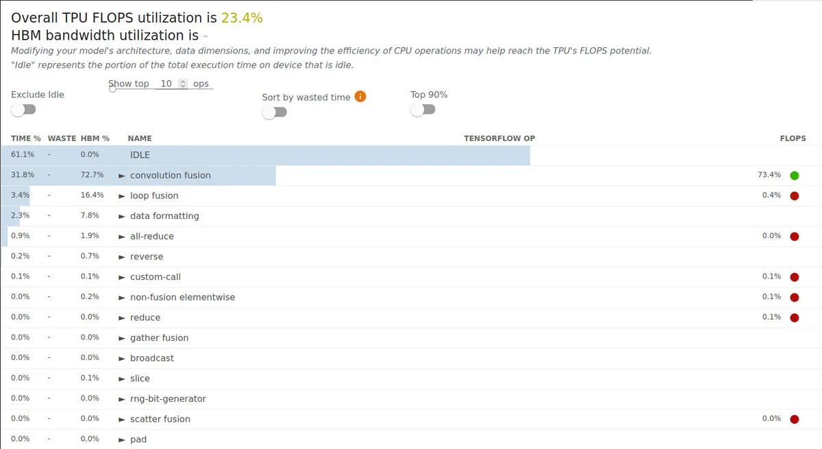
Using larger batch sizes to hide CPU bottleneck
Using a large batch size is the first thing that most TPU performance guides tell you to do, but this optimization took me a while to find specifically when training the DM because I had nearly no idle time training the VAE with a per-device batch size of 32 (batch size of 256 over all eight chips), but had 42.7% idle time when training the DM with the same batch size. This is because XLA requires a graph of the training loop to be traced for every training step [10], which uses up some CPU time. Since the VAE was a relatively simple model, tracing time was not an issue, but the DM was significantly larger, so I needed much larger batch sizes to reduce idle time. At the time, I didn't know about that the CPU time was caused by tracing, but I found out that increasing the batch size increased the TPU execution time but not the CPU time, so I just pushed the batch size to as large as I could. I eventually settled on a batch size of 128 (although I got up to 192) because it was the largest batch size which I could train on without running out of CPU memory while compiling. With a per-device batch size of 128, I had only 12.1% idle time, which was far better than the 42.7% I had earlier.Along with the more TPU-friendly models, training utilizes TPUs much more effectively, going from 23.4% to 55.3% FLOPs utilization at a per-device batch size of 128.
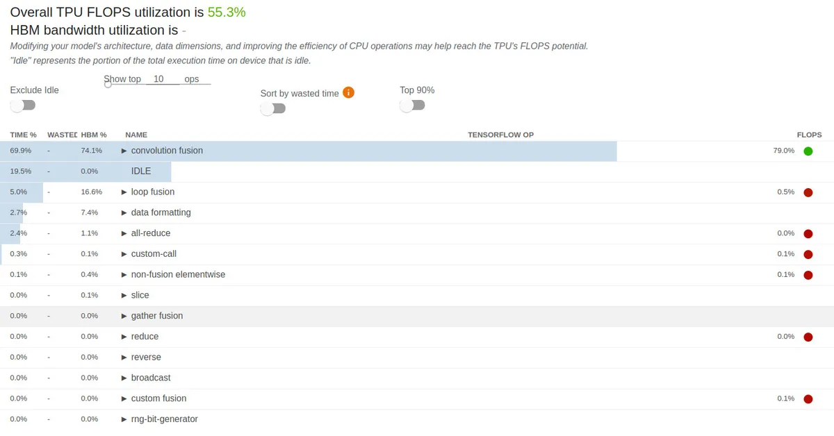
Better model utilization now. But 19.5% of training time is idle, we can still do better!
I'm shocked by the fact that I was able to train a batch size of 128 with only 16 GiB of memory per chip, XLA is crazy effective. Here are some memory logs:
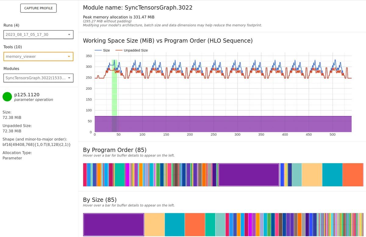
Memory viewer for the CLIP embedder. For a batch size of 128, it only uses 330 MiB!
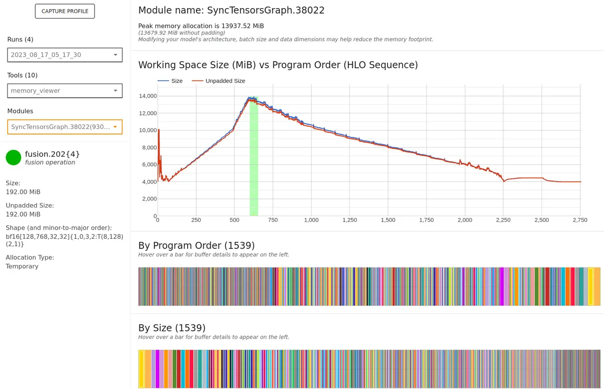
Memory viewer for the VAE and DM. For batch size 128, these use almost 14 GiB of memory.
Using torch.compile(..., backend='torch_xla_trace_once') for the VAE and CLIP embedder
January 5, 2024 update: I think you're supposed to set the backend to 'openxla_eval' now.
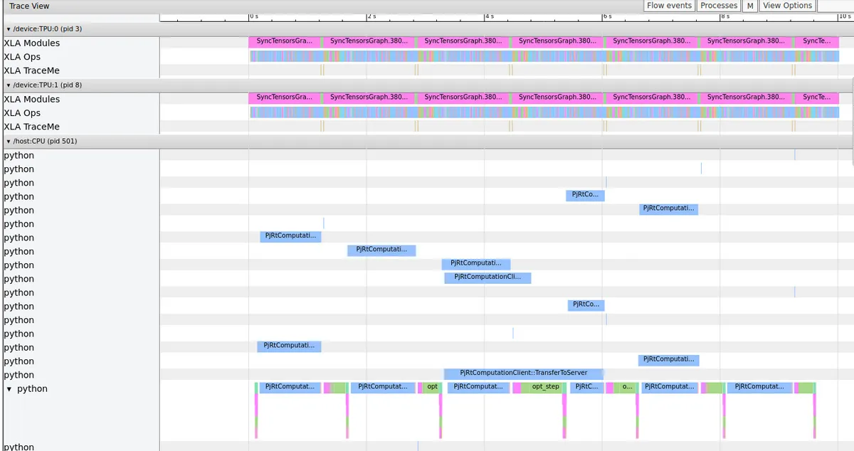
While I removed most of the idle time by logging less frequently, I noticed some idle time on some steps that had didn't seem to be caused by logging (no TransferFromServer calls). Rather, the idle time seemed to have been caused by some bottlenecks:
More trace viewer snapshots showing idle time even without TransferFromServer (loss logging calls).
After some searching, I found a GitHub issue with a similar problem. Apparently, the problem was that there was a CPU bottleneck from tracing, causing the idle time. The proposed solution was:
If this model is tracing bound, I think maybe we should give dynamo a try
So I tested this idea with a full-sized VAE, a small CLIP embedder (CLIP-base-32), and a tiny DM. I tried to wrap the DM with torch.compile (which uses TorchDynamo) and ... it did not work. The program would just keep hanging, even in the debug mode, so I tried compiling just the VAE and CLIP embedder which gave some results (2.7 steps/s → 2.9 steps/s; each step became faster 0.0255 s faster).
This was a bit disappointing since a training step with the full-sized DM took around two seconds. This optimization's speedup should've been unrelated to the DM's size since I didn't compile the DM, so I expected this speedup to be negligible (about 0.0255 / 2 = 1.27% speedup) when training. Unsatisfied by a 1% speedup, I continued attempting to compile the DM with TorchDynamo. I eventually got it to train (only when using one TPU core) but I had to reduce the batch size 8x (128 → 16 per-device batch size) to get the thing to fit into memory. And I was running out of Kaggle TPU time, so I just ran a training run using torch.compile only on the VAE and CLIP embedder.
Yet when I resumed training with what I expected to be a 1% speedup, I got a 25% speedup, with step time going down to 1.6 s/step. Apparently torch.compile made the DM forward, backward, and optimizer step run WAY faster in the Python processes (I'll stress it again, I didn't compile the DM or the optimizer)! I don't know why, but I'll take it.
Trace viewer when compiling the VAE and CLIP embedder. Look, no idle time!
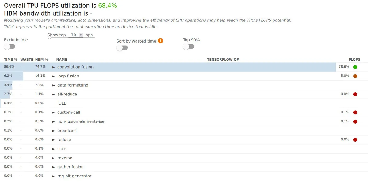
FLOPs utilization goes from 55.3% without compiling to 68.4% when compiling the VAE and CLIP embedder with torch.compile. Actually, I think FLOPs utilization is closer to 65% since this snapshot didn't profile any loss logging which adds some idle time.
Optimization Summary
Micro-optimizations (no FLOPs utilization increases recorded for these)
- Logging loss every 32 steps
- Writing custom multi-head attention class
- Replacing GELU with SiLU
- Better attention head splitting
- Reduce usage of torch.split
- No biases in transformer blocks
Macro-optimizations
| Optimization description | FLOPs utilization (%) | Idle time (%) | FLOPs utilization increase over previous optimization | FLOPs utilization increase over baseline |
|---|---|---|---|---|
| baseline (small models, per-device batch size=32) | 23.4 | 61.1 | 1.00 | 1.00 |
| TPU-friendly models + per-device batch size=128 | 55.3 | 19.5 | 2.36 | 2.36 |
| Compile VAE and CLIP embedder with torch.compile | 68.4 | 6.2 | 1.24 | 2.92 |
Strange Bugs
Note: These are also ordered from when I found them.
XLA_USE_BF16=1 destroys training
Mixed precision is faster. Using just bfloat16 can speed up TPU training by up to 60% [9], and PyTorch allows this by setting the environment variable XLA_USE_BF16=1 [10]. However, while the model forward and backward passes work fine in bfloat16, the noise schedule in the DM (as well as the DDIM sampler) requires the float32 precision, which I realized when all of the DM outputs was black after some training. Inspecting many components of my training script, I eventually found that the noise variances in the noise scheduler would differ between bfloat16 and float32, which messed with the signal and noise variances for each step.
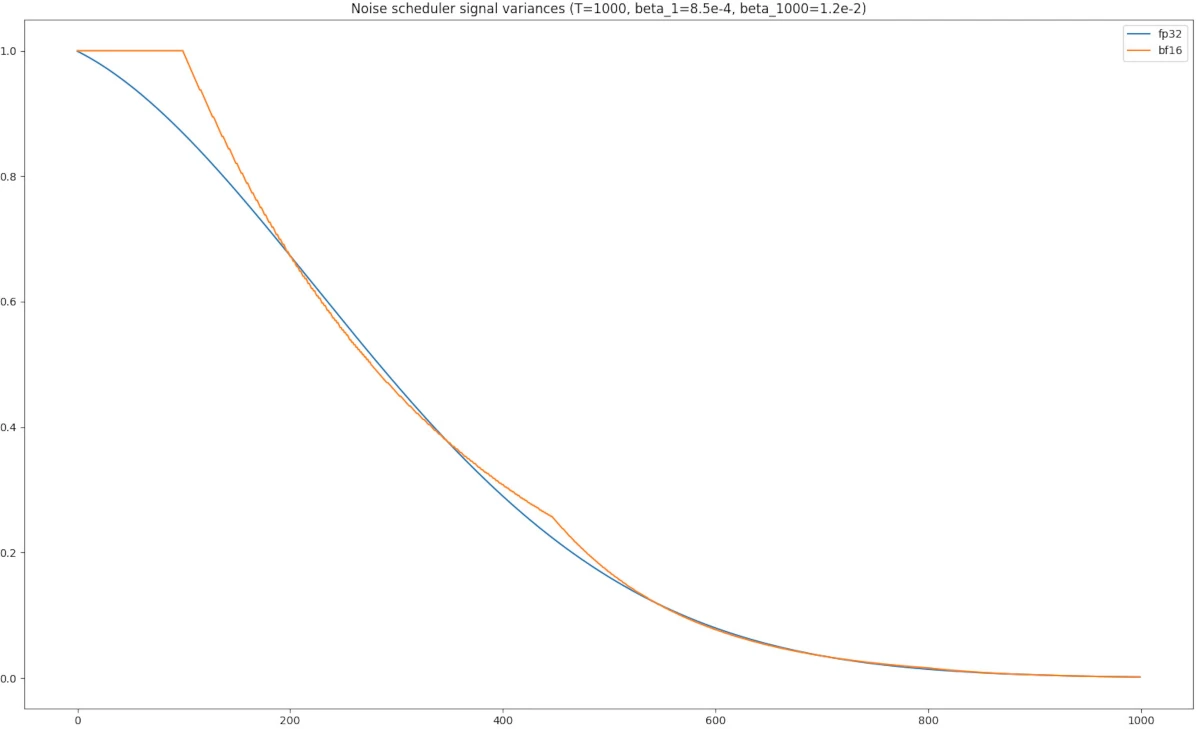
Using bfloat16 results in strange noise scheduler behavior when compared to float32.
Specifically, in the DDIMSampler code, there are lines:
self.betas = 1 - self.alphas
(omitted code)
beta_ratio = self.betas[t-1] / self.betas[t]
The graph above shows self.alphas, and notice in the bf16 graph, there are multiple steps t where self.alphas[t] = 1, meaning that self.betas[t] = 0. This means that there would by a divide-by-zero error in beta_ratio, which would cause any tensors that use beta_ratio to be corrupted (such as the outputs of the DDIM sampling).
To deal with this, I set the environment variable XLA_DOWNCAST_BF16=1, which gives me access to float32 precision by casting a tensor to torch.double [10]. I suppose there are multiple ways to deal with this problem, but this was the first one that came to my mind, and since the noising/denoising computation is negligible compared to the forward/backward passes, I didn't worry too much about optimizing this.
Another related problem (which I figured out far later) was that normalization had to be set to fp32 for training to run smoothly. I encountered this problem when training the DM using a trained VAE with 32 groups in the GroupNorm layer (to match with the original code; I originally had eight groups in the GN layers as I started this project when my local GPU only had 2 GiB of VRAM (side note: GiB = 2^30 bytes = 1024 MiB, GB = 10^12 bytes = 1000 MB) so my models had to be scaled down a lot). Training would run smoothly for the few first thousand steps or so, but then randomly collapse. This is seen in train3a-c-56. I thought this collapse had to do something with the GN layers, so I dropped the number of groups (only in the DM, not the VAE) to eight. That's train-3a-d-58 (so no, it did not fix the problem). Reading through the original papers again, I realized that they were training their models with AdamW rather than plain Adam. I added AdamW for train3a-e-69. Finding the root problem for this collapse would be a bit trickier than I originally thought.
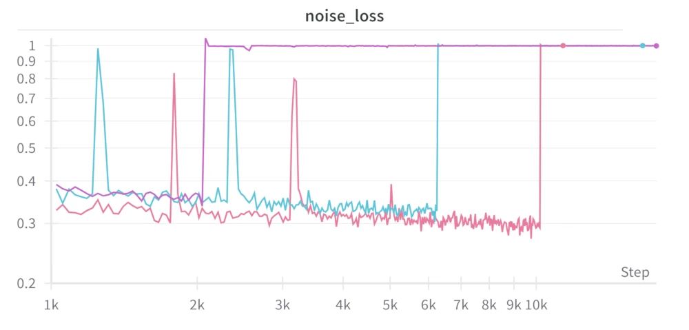
Model collapse with GN (groups=32, groups=8) and AdamW. Something else is the problem...
I don't have this documented, but I remember looking through the activations of each layer of a collapsed model to see what may be going wrong. One, I found out that the norm of the activations kept increasing exponentially after each layer in the collapsed model. Two, the activations all had constant values. Because of the constant value activations, after the last normalization layer, the normalized activations would turn into all zeros, which would yield a loss of 1 (as the DM loss function mean((eps - DM(x, t))^2) where eps is the target noise sampled from a normal distribution, x is the noised image input, and t is the timestep is equal to 1 when DM(x, t) is always equal to 0).
This confused me. Shouldn't the GN keep the activation norms within reasonable levels? I verified that the normalization layers were in fact doing their job, so I was stumped, but I felt that the problem still laid in the normalization layers in some way. By educated guesses and trial and error, I decided to test out a possible problem. What if the mean of the activations is relatively high but the variance is relatively low? In this case, I wasn't completely sure what was going to happen, but I felt that the low precision of bf16 might've been a problem. Here's some code that roughly describes what I did:
def norm(x): return (x - x.mean()) / x.std()
x = torch.randn((10,), dtype=torch.bfloat16)
x1000 = x + 1000 # norm(x1000) should equal norm(x) which is roughly equal to x
But if you run the above code, you get some weird result like tensor([0.0000, 0.0000, 0.0000, 0.0000, 0.0000, 0.0000, 0.0000, 0.0000, 3.1562, 0.0000], dtype=torch.bfloat16). Aha! Precision is a problem in this case! So I tried running the GN layers in fp32...
class StableNorm(nn.Module): # runs GroupNorm in FP32 because of bfloat16 stability issues when x is large but with small variance (i.e. x = 100)
    def __init__(self, num_groups: int, num_channels: int):
        super().__init__()
        self.norm = nn.GroupNorm(num_groups, num_channels).double() # under XLA_DOWNCAST_BF16=1, double is casted down to fp32

    def forward(self, x):
        return self.norm(x.double()).float() # under XLA_DOWNCAST_BF16=1, float is casted down to bf16
And the model collapse stopped! Also, performance didn't get significantly worse from this, so that's nice.
Using TFRecordDataset causes train function to hang before training begins
I wanted to use TFRecords for my dataset since TPUs have extremely high throughput and TFRecords are the recommended way (as opposed to an image folder, webdataset, etc.) to prevent a data bottleneck. I've worked with Tensorflow's TFRecordDataset in the past so I thought that it would work, but it just caused my training loop to hang. It might have something to mixing TF and PyTorch, but I knew that I wouldn't be able to come up with a fix for this problem myself, so I looked for other ways to load TFRecords in PyTorch. I tried looking into Torch XLA [20] to see if it had the solution, but it just didn't work for me. After some more looking, I found [21] which offered what I needed (this is unrelated, but the library has sixty closed issues and no open issues! I respect that so much.). No more hanging! I realized later that the dataset was returning the same batches across each of eight TPU workers, but that was easily fixed by initializing the dataset in each of the TPU workers with different sections of the dataset.
Einops sometimes doesn't work
Einops is a cool library to make tensor rearrangements and reductions simpler, and I tried using it, but it caused some errors during compilations. So I just used PyTorch's permute, reshape, and contiguous operators to do what Einops was supposed to do.
Setting scale_factor argument when upsampling images slows training
When I first got VAE training to work on TPU, I first noticed that step times were extremely slow after the first few steps which indicates that something was wrong in my training. The PyTorch XLA docs have some good resources [22] to find out where to find the causes of any slowdowns using PyTorch metrics, and when I tried running metrics on my slow code, I noticed many calls to the CPU op for upsampling. Digging through Github for a solution to this problem, I found [23] which solved the problem for me. All I had to do was change my upsampling code as shown below:
def forward(self, x):
    # BEFORE
    #return self.conv(F.interpolate(x, scale_factor=2.0, mode='nearest'))

    # AFTER
    _B, _C, H, W = x.shape
    return self.conv(F.interpolate(x, size=(H*2, W*2), mode='nearest'))
After that, there were no ops that ran on the CPU during training, which made training run at a reasonable speed.
Not logging loss with loss.item() causes OOMs
I don't know why my solution worked. But I knew that TPU training would be fine for a couple of epochs, then run out of memory, and then when I set loss.item() when logging metrics to W&B, the problem went away.
More CPU memory is used up every epoch
In my first few training runs, I noticed that my CPU memory stepped down every epoch (emphasis on epoch; the CPU memory stayed constant between different steps on the same epoch as well as would not drop if I set each epoch to have infinite steps). The only thing I could reason was that my dataloader was being refreshed every epoch, so why don't I instead reuse the same dataloader object for every epoch? Here's roughly what I did in code:
# BEFORE
def train_loop(self, epochs=1, steps_per_epoch=-1, save_every_n_epochs=1):
    for epoch in range(epochs):
        loader = pl.MpDeviceLoader(self.loader, self.device)
        for step, (imgs, _captions) in enumerate(loader):
            # training step
            if step == steps_per_epoch - 1:
                # save models, log images, etc.
                break

# AFTER
def train_loop(self, epochs=1, steps_per_epoch=-1, save_every_n_epochs=1):
    loader = pl.MpDeviceLoader(self.loader, self.device)
    for step, (imgs, _captions) in enumerate(loader):
        # training step
        if step == steps_per_epoch - 1:
            # save models, log images, etc.
            epoch += 1
            if epoch == epochs:
                break
Training from a model checkpoint is slower than training from random initialization
During the first epoch, the VAE would train at 2.08 steps/s, but when I resumed training from a model checkpoint, the training speed dropped to 1.13 steps/s, about 54% of normal speed. So I knew that this problem laid in the loaded model, and by running the Tensorboard profiler, I found out that the optimizer step took a long time on the CPU, resulting in lots of TPU idle time. What I found out was that there was a large number of tensors being moved from the CPU to the TPU during the optimizer step, which is slow.
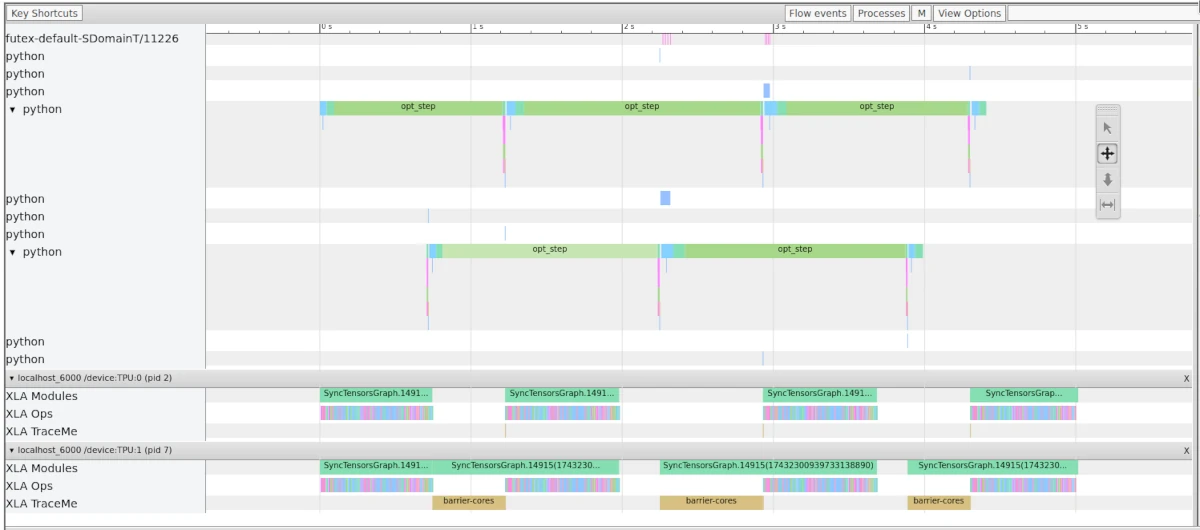
BEFORE FIX: Notice that the TPUs are idling and its cause: opt_step (correlating to an opt.step() call) has really big Python overhead. Something is up with the optimizer! (Note: this actually runs at around 1.45 steps/s, I don't know why this run is faster than the 1.13 steps/s run where I first saw this problem, but it highlights the same issue)
I initially tried to move all optimizer parameters to the TPU when I initialized my trainer, but this didn't work for some reason. Thankfully, the fix was pretty easy. I sent the model to the TPU, and then I made my optimizer using the TPU model's weights. Here's what the fix looks like in code:
# OLD
def load_models(device='cpu', lr=1e-4, ckpt_path=None):
    vae = VAE().to(device)
    disc = Discriminator().to(device)
    vae_opt = Adam(vae.parameters(), lr, (0.5, 0.9))
    disc_opt = Adam(disc.parameters(), lr, (0.5, 0.9))

    if ckpt_path is not None:
        ckpt = torch.load(ckpt_path, map_location=torch.device('cpu'))
        vae.load_state_dict(ckpt['vae_state_dict'])
        disc.load_state_dict(ckpt['disc_state_dict'])
        vae_opt.load_state_dict(ckpt['vae_opt_state_dict'])
        disc_opt.load_state_dict(ckpt['disc_opt_state_dict'])
    (omitted code)

# NEW - I was thinking of finding a nicer way to write this fix in code, but I didn't care enough
def load_models(device='cpu', lr=1e-4, ckpt_path=None):
    vae = VAE().to(device)
    disc = Discriminator().to(device)

    if ckpt_path is None:
        vae_opt = Adam(vae.parameters(), lr, (0.5, 0.9))
        disc_opt = Adam(disc.parameters(), lr, (0.5, 0.9))
    else:
        ckpt = torch.load(ckpt_path)
        vae.load_state_dict(ckpt['vae_state_dict'])
        disc.load_state_dict(ckpt['disc_state_dict'])
        vae = vae.to(device)
        disc = disc.to(device)

        # now the optimizers will be initialized with on-device parameters
        vae_opt = Adam(vae.parameters(), lr, (0.5, 0.9))
        disc_opt = Adam(disc.parameters(), lr, (0.5, 0.9))
        vae_opt.load_state_dict(ckpt['vae_opt_state_dict'])
        disc_opt.load_state_dict(ckpt['disc_opt_state_dict'])
    (omitted code)
And when I profiled the code, here's what it looked like:
Calling loss.item() on only the master ordinal causes training to hang
Funny how loss.item() seems to fix one problem but causes another one. The reason this happened was that I was logging my metrics, I only called loss.item() for the master TPU ordinal (there are eight ordinals as I was training on eight TPUs). The problem is that loss.item() executes the XLA graph (AKA the TPU actually does computation after this call) [10], but since I only call loss.item() on one out of the eight TPU workers, seven of the TPU workers will be extremely ahead the single worker that was actually doing computation. This lack of sync between workers then causes the training loop to hang there is an operation where all TPU workers have to sync (e.g. making an optimizer step, saving models, etc.). To fix this problem in my code, I just had to change the position of one line of code when logging my metrics:
def log_step(self,
    log_metrics: dict, step: int,
    epoch: int, epochs: int, steps_per_epoch: int, pbar
):
    log_items = {k: v.item() for k, v in log_metrics.items()} # AFTER - no training hang
    if xm.is_master_ordinal():
        # log_items = {k: v.item() for k, v in log_metrics.items()} # BEFORE - causes training hang
        if self.wandb_run is not None:
            wandb.log(log_items, step=self.global_step)
While this was definitely a problem where I knew enough info beforehand to avoid, this took me a surprisingly long time to locate. This was because:
The training hang would always happen when I was saving my model, so I thought my problem had to do with saving the model. But as you can see above, the root of this model is unrelated to model saving, so I was spending a lot of time focusing on the wrong part of my code.
At this point, I had little experience debugging programs that would stop and idle. I've worked with programs that would freeze because it would run into an infinite loop, but that wouldn't make the CPUs start idling. I didn't know why a program would start doing nothing, so to me, the root of this problem could've been anywhere and thus I looked everywhere in my code for potential problems, mostly in areas with no issues. Also because of the lack of errors, I spent a lot of time on runs where I just printed out extra messages before freezing to help isolate the problem.
Since XLA takes a while to compile big models, I tried debugging with small models. However, when I did this, I couldn't reproduce the training hang.
All in all, it took me 40 runs according to W&B to fix the problem, although I usually turned off W&B when I encountered bugs that were hard to fix, so it probably took me even more runs to find the solution. I also went through a lot of Github issues to locate the problem, and I think [24] was the one that helped me the most to understand how to deal with this problem.
The same model in different parts of training use different amounts of CPU RAM
When training the DM, my sessions usually hit a peak between 260 (train3e-a-78) and 290 (train2_pt4-24) GB (out of 330 GB) of RAM usage but there were two runs where I somehow used up like 320 GB of the TPU session's available RAM even though I didn't change the code (train2_pt2-22/23). I don't recall fixing this problem. On the runs where I used 320 GB of RAM, all I did was continue training and saving the model. When I loaded from the saved model in a different session, it just stopped using so much RAM, which is shown in run train2_pt4-24. And if I were to completely run out of RAM on a session, I'd probably reduce the batch size, train the model for a bit, save it, then restart the session and load the saved model with the original batch size.
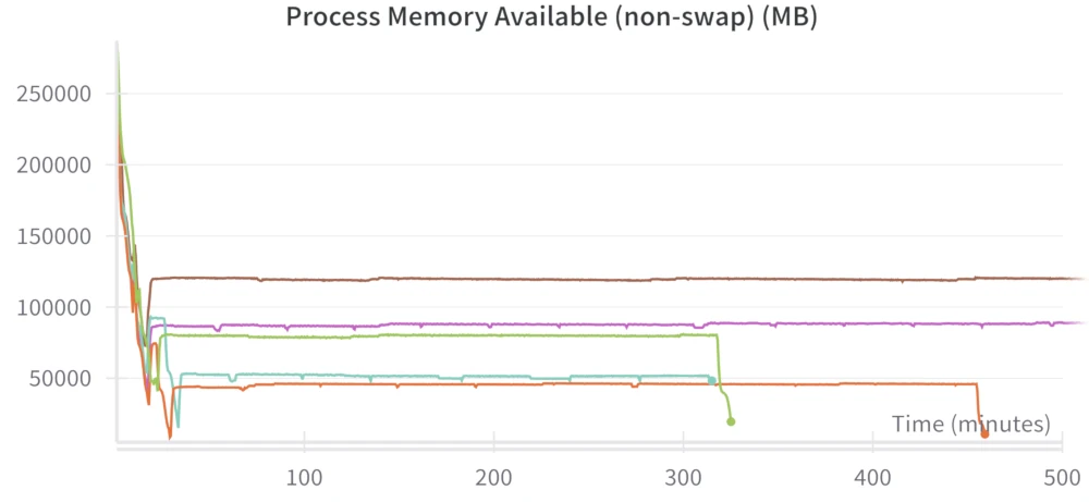
Some training runs eat up more free memory than others for some reason. The only changes between these runs are the checkpoints used.
Things That Didn't Work
Tokenizing captions in DataLoader
I tried to tokenize captions in the DataLoader in an attempt to remove some overhead as data loading and model training can happen together. But whatever I tried, it never made my training any faster and it made my code uglier so I stopped trying.
Training fast with FSDP
The MosaicML Stable Diffusion report [25] described using FSDP to get a 17% speedup in training even though FSDP is meant for models far larger than Stable Diffusion. They got their speedup since they found that their optimizer step was quite slow because of all of the gradient communication over the 128 GPUs they were training across. To lower this communication, they used FSDP to shard the model optimizer states across each GPU so each GPU sends and receives a smaller amount of data. I knew that my scenario was different as I was training over eight TPUs which are essentially on the same chip (rather than connected over a relatively slow network), so gradient communication should be negligible. But I wanted to try FSDP anyway just in case there were any sizable speedups and also just to learn more about FSDP. It was a pain to set up, and even when I finally got the model training, it was really slow (about 2-3x slower than normal). I tried to find a solution to this slowness, but I couldn't, so I just stopped trying to use FSDP.
Non-sinusoidal timestep embeddings
I remembered reading the Keras tutorial on DDIMs [18] to understand the code of diffusion models and the author left a note about how sinusoidal timestep embeddings were crucial for good performance. For some context, the timestep sinusoidal embedding is calculated as:
def sinusoidal_timestep_embedding(timestep: int): # timestep between 0-999 inclusive
    sinusoid_emb = sinusoidal_embedding_fn(timestep) # takes in int, returns length 256 vector
    x1 = Linear(256, 1024)(sinusoid_emb)
    x2 = SiLU(x1)
    x3 = Linear(1024, 1024)(x2)
    return x3
Here's why I thought a vanilla embedding would work. We already know all possible timesteps (0-999 inclusive), and the sinusoidal embedding function is deterministic, so we already know all outputs of sinusoid_emb. And since the input for the first linear layer is already known, we can treat x1 as either a matrix multiplication of a learnable matrix with a constant one OR as just a learnable matrix. Same logic applies for x2 and x3, which allows us to rewrite the whole sinusoidal timestep embedding as a single learnable embedding of shape (1000, 1024).
But as I said, this didn't work. When I was training my DM with the single learnable embedding, my loss was going down, but the image quality never got good. I was starting to think more about the Keras tutorial's note on sinusoidal embeddings, as at this point I was sure that everything else about my network was correct. Eventually, I realized my method was flawed for two reasons:
- I was effectively reducing my batch size on the embedding by a factor of 1000. To clarify, with a batch size of 256, and assuming no repeated timesteps, I would only have gradients for 256 rows of the embedding per batch. But of the embeddings that were used in the forward pass, since each embedding was used for only one element within the batch (effective batch size of one if a gradient was received and a batch size of zero otherwise), its gradients would be very noisy. For the original sinusoidal timestep embedding, the learnable parameters rest in the linear layers which means that all of the parameters would be used for each element within the batch (effective batch size of 256).
- Because the different timesteps represent slowly changing levels of noise strength in the input image, it makes sense that rows of timestep embedding that are spatially close to each other (e.g. row 10 and row 11) should have similar element contents (i.e. the vector distance between the rows should be close to 0) since spatially close rows represent similar levels of noise strength. A vanilla learnable embedding does not have this inductive bias whereas the sinusoidal embedding does, which means that training should be much easier with the sinusoidal embedding.
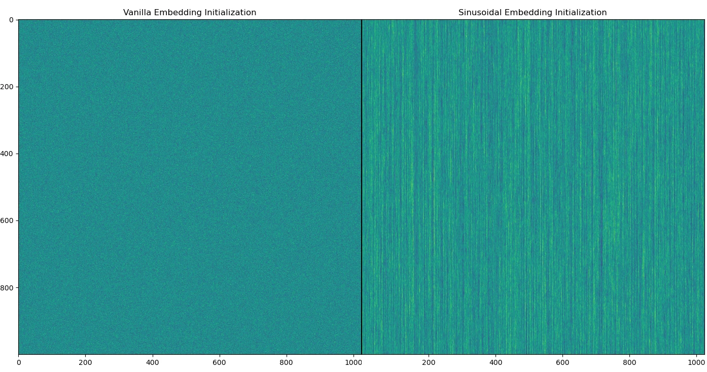
The k-th row on both images represents the activation values of each embedding for t=k. Notice how the different rows in the vanilla embedding are completely independent of each other and how this is not the case for the sinusoidal embedding.
Below shows a comparison of the DM outputs where the loss is similar and the main difference is the embedding. Note that I said "similar loss" and not "similar training time" since the training run with sinusoidal embeddings (~70k steps to mse=0.267) trained more than twice as quick as the run with vanilla embeddings (~164k steps to mse=0.267):
Using vanilla embeddings
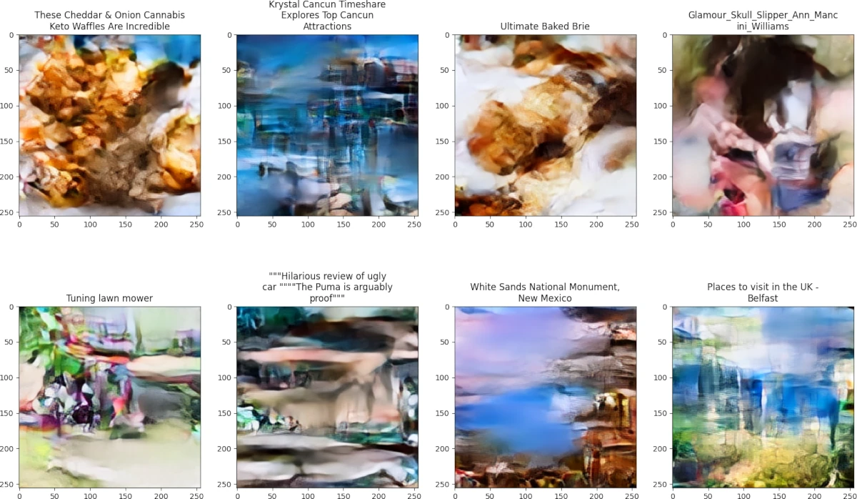
All the samples from the vanilla embedding run look like paint splotches.
Using sinusoidal embeddings
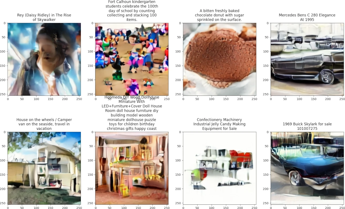
The house and car samples look vaguely like houses and cars, a clear win for the sinusoidal embeddings.
Training Progress
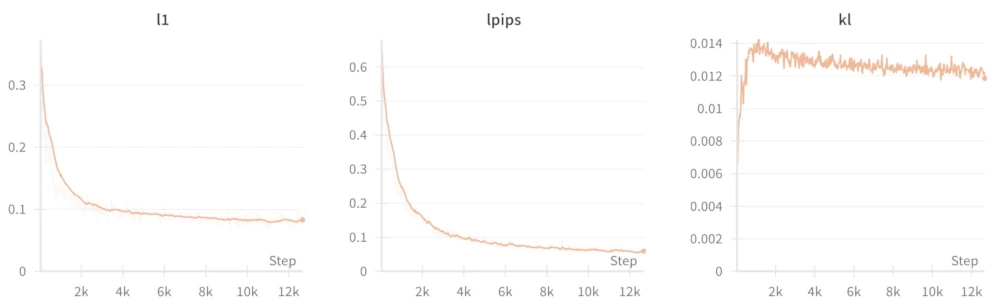
VAE
DM
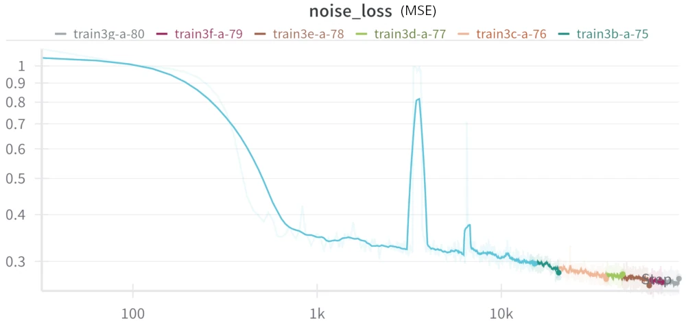
Note: this is a log-log plot
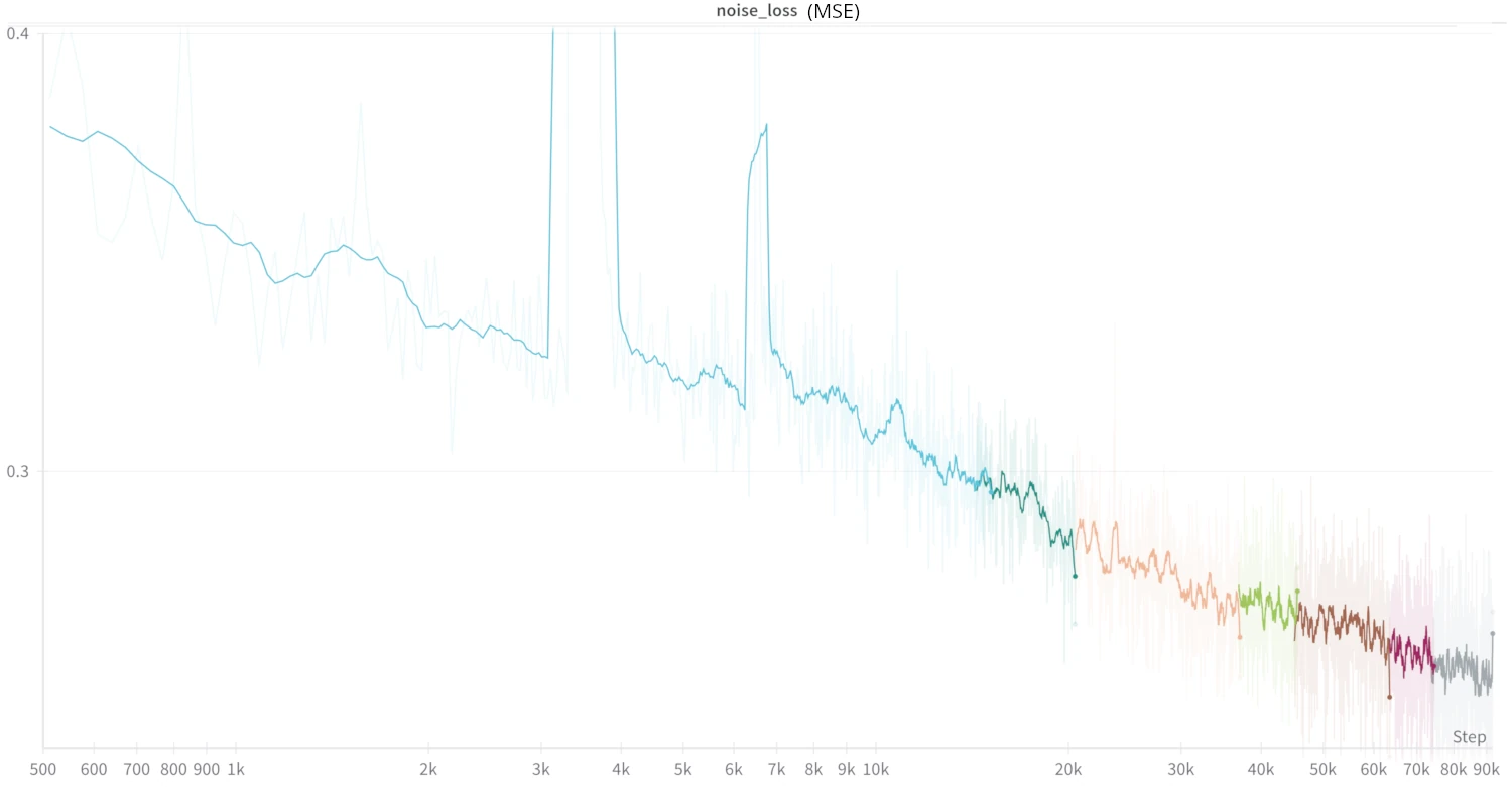
The above plot but ignoring the high-loss areas (after 500 steps, clipping the moment around 3k steps where the loss temporarily spiked). Loss steadily went down at 90k steps which means I could've gotten better results by training longer, but I stopped because I got bored of waiting.
Conclusion
And that's it! Even though I was replicating an already open-source project, I learned a lot from doing this. Some takeaways:
- Read the tutorials carefully. Many of the issues I faced were things that that I glossed over in tutorials.
- Make your debug runs as small and focused as possible. I used up so much time debugging as I would spend 30 minutes of waiting, get an error message, change one or two line of code, and repeat. For example, if you can replicate the issue with a smaller model, use a smaller model. If you can replicate the issue using only one device rather than eight, use only one device. You get the idea.
- Document your work. It's good to do this in case you encounter the same problem in the future so you can refer to how you fixed the problem. I documented my work by writing descriptions on each W&B run of what I changed and of any new issues that happened in the run. I also saved my training code and uploaded it on W&B for every run. Making this report would've been impossible if I didn't do both of these.
- Use built-in debugging tools and profilers.
References
- TPUv3 Architecture
- P100 Datasheet
- T4 Datasheet
- Scaling Vision Transformers to 22 Billion Parameters
- PaLM: Scaling Language Modeling with Pathways
- FlashAttention GitHub
- What is GELU?
- GLU Variants Improve Transformer
- TensorFlow Mixed Precision Guide
- PyTorch XLA Guide
- TensorFlow TPU Performance Guide
- Locality of Reference Wikipedia Article
- Cache-Blocking/Tiling Matrix Multiplication Tutoria
- Memory, Cache Locality, and Why Arrays Are Fast
- Attention Is All You Need
- LDM Github - diffusionmodules/model.py
- x-transformers Github - README.md
- Keras DDIM Tutorial
- SDXL Technical Report
- Torch XLA TFRecordReader
- Vahid Kazemi's TFRecord Library
- PyTorch/XLA: Performance debugging on Cloud TPU VM: Part I
- CPU Upsampling when scale_factor != 1.0
- Training hang in PyTorch XLA
- MosaicML Stable Diffusion Report
Changelog
- August 27, 2023: Article made
- January 5, 2024: Added note about xla backend names changing for torch.compile
- September 2, 2024: Added cover image, reorder paragraphs from optimization logs to make more sense, published this article to my site
- September 3, 2024: Minor formatting changes